Theoretical Mechanics
1.2 Mechanics of Multiple Particles:
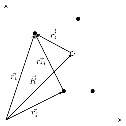
Vector notations for points of mass and the center of mass.
1.3 Bindings:
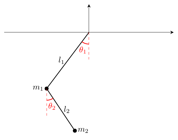
Double pendulum.
1.4 lagrange multipliers:
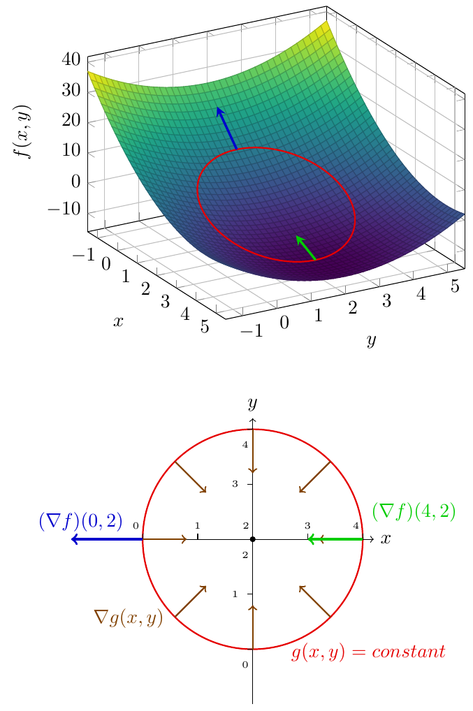
We seek to find the maxima and minima of $f(x,y) = (x-3)^2 + (y-2)^2 - 3x$ subject to the constraint $(x-2)^2 + (y-2)^2 = 4$, i.e., $g(x,y) = 4$. This constraint circle is shown in red on the surface $(x, y, f(x,y))$ in Figure~1. Maxima on this restricted curve do not require $\nabla f = 0$. Indeed, the non-zero gradient vectors in the extrema are drawn here, tangent to the surface along the curve (blue and green vectors). In Figure~2 ($xy$-plane), notice that only at extrema is $\nabla f$ parallel to $\nabla g$. The gradient $\nabla g$ is always perpendicular to the level curve $g(x,y)=4$ (brown arrows). Thus, a sufficient condition for extrema is $\nabla f = \lambda \nabla g$, where $\lambda$ are the Lagrange multipliers. This gives, together with the equation $g(x,y) = 4$, a system that can be solved for the extrema.
1.6 Atwoods Machine:
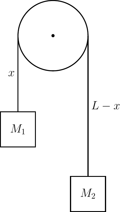
Atwood’s machine.
2.6 Conservation Properties and Symmetry Properties:
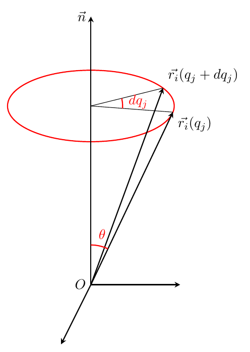
Change of position vector under rotation.
4.4 Euler angles:
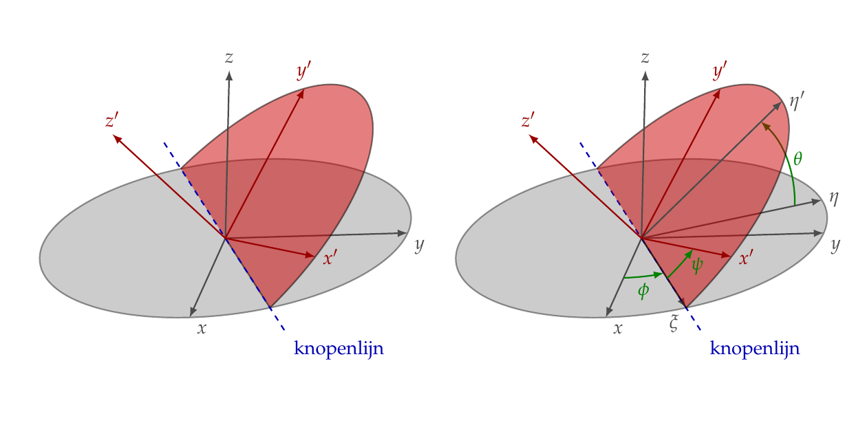
The rotations defining the Eulerian angles.
4.7 Finite Rotations Detail:
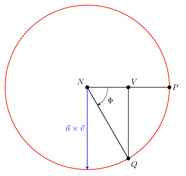
Detailimage of the circle on which the rotation takes place.
4.7 Finite Rotations:
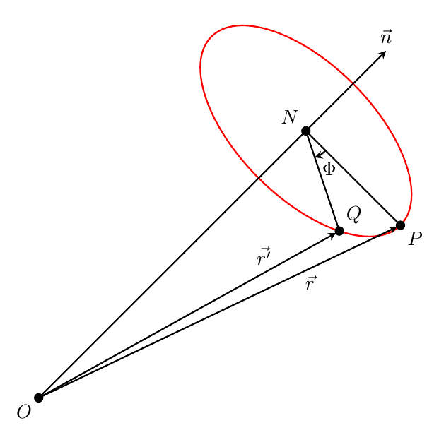
Finite rotation around an axis.
4.8 Infinitesimal rotations:
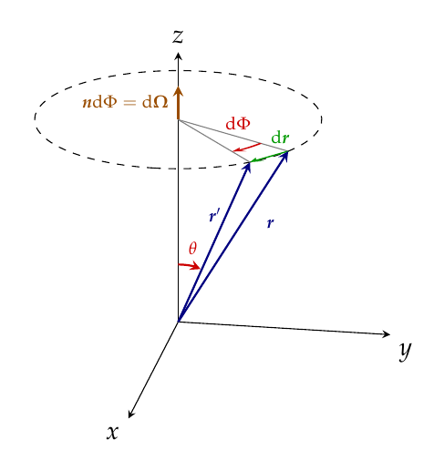
Change in a vector $\boldsymbol{r}$ produced by an infinitesimal clockwise rotation $\mathrm{d}\Phi$ of the vector.
4.9 Rate of change of a vector:
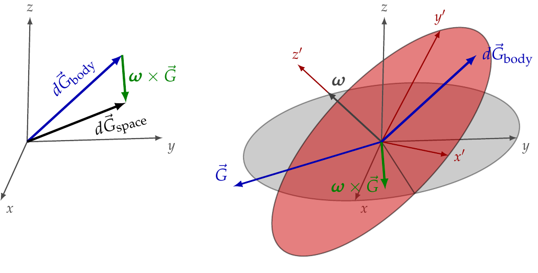
Rate change of a vector $\vec{G}$, as perceived by an observer in the fixed body frame: $d \vec{G}{body}$ (right) and in the space frame: $d \vec{G}{space} = d \vec{G}_{body} + \pmb{\omega} \times \vec{G}$ (left). The $z’$ axis is chosen such that it aligns with $\pmb{\omega}$.
4.10.1 coriolis on sphere:
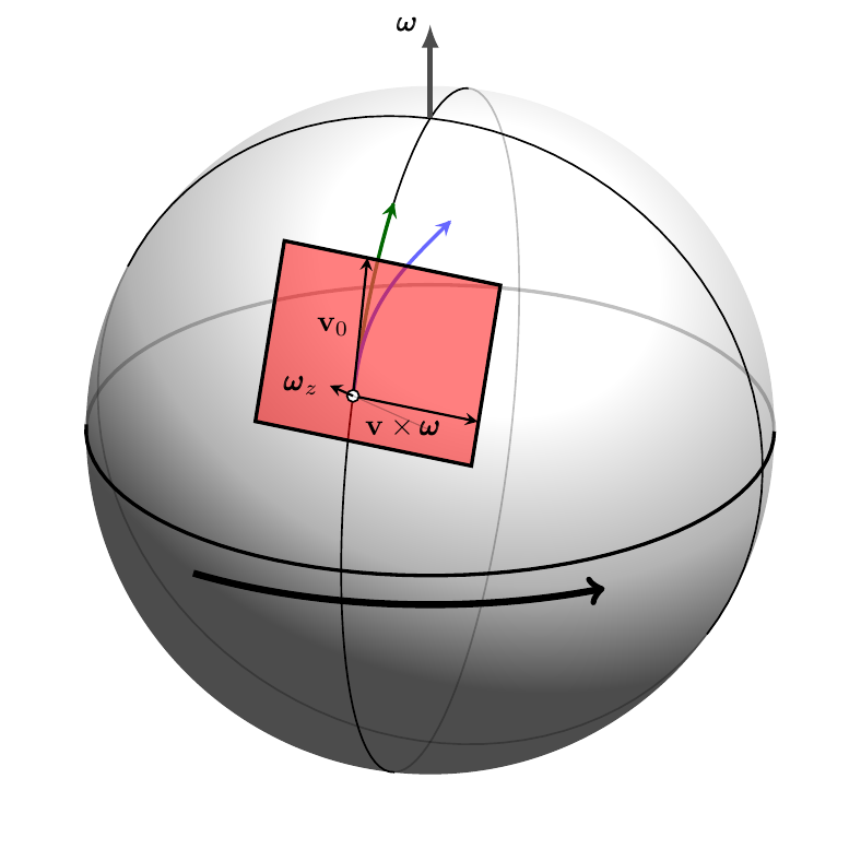
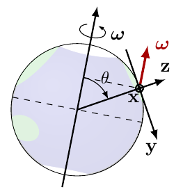
Coriolis effect for an object moving northward on a rotating sphere. The green trajectory shows the motion for when the Coriolis effect is neglected, while the blue trajectory takes the Coriolis effect into account.
4.10.2 coriolis effect local:
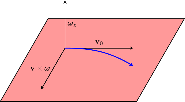
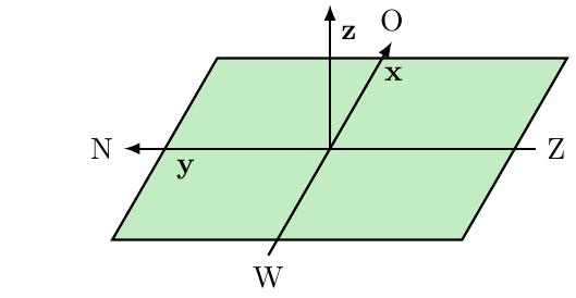
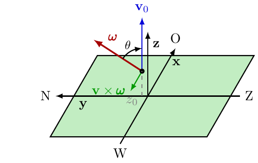
Local view of Coriolis deflection (blue) for an object moving northward.
4.10.3 centrifugal force:
4.10.3 coriolis sphere sol:
4.10.3 coriolis sphere task:
4.10.4 coriolis local task:
4.10.4 coriolis local sol:
4.10.4.1 coriolis forces northern hemisphere:
4.10.4.2 coriolis forces northern hemisphere:
4.10.5.1 coriolis forces southern hemisphere:
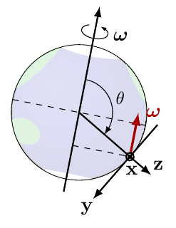
4.10.5.2 coriolis forces southern hemisphere:
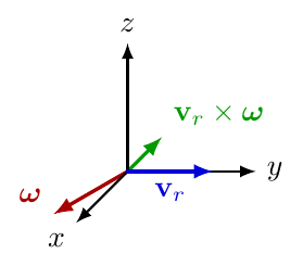
4.10.6 coriolis effect vortex:
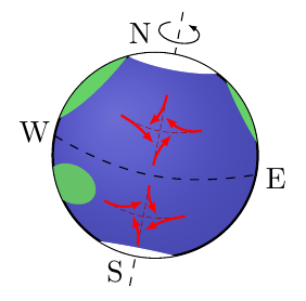
4.10.7.1 coriolis NH vertical velocity:
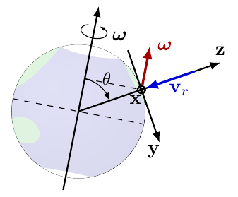
4.10.7.2 coriolis NH vertical velocity:
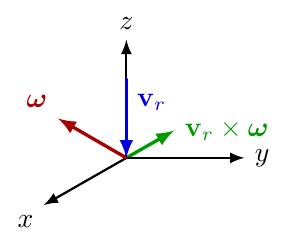
4.10.8.1 coriolis SH vertical velocity:
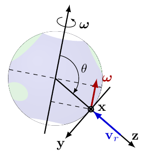
4.10.8.2 coriolis SH vertical velocity:
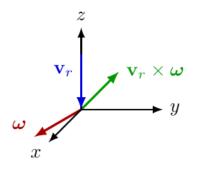
5.2 traagheidstensor balk 2D visualisatie:
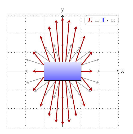
Graphical representation of the relationship between the angular velocity vector $\pmb{\omega}$ (gray) and the angular momentum vector $\pmb{L}$ (red) for a rectangular beam with inertia tensor $\mathbf{I}$. The directions of $\pmb{L}$ and $\pmb{\omega}$ do not coincide due to the anisotropy of the inertia tensor. The rectangular beam has dimensions 2, 1, and 0.2 along the x, y, and z axes respectively and is homogeneous in density.
5.3 visual proof parallel axis theorem for pointsymmetrical bodies:
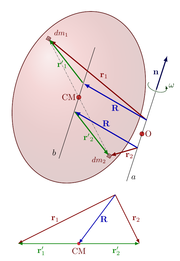
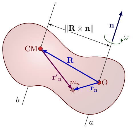
One wants to prove that $I_a = I_b + M ( \vec{R} \times \vec{n} )^2$. For this, one can consider the 3D figure. Notice that all vectors in green, blue and red are perpendicular to the vector $\vec{n}$. For a point-symmetrical, homogeneous body, it is enough to show that for two point masses $dm_1$, $dm_2$, $dI_a = dI_b + dI_{CM}$. Here, $dI_a = dm_2 r_2^2 + dm_1 r_1^2 = dm_1 (r_1^2 + r_2^2)$, $dI_{CM} = 2 dm_1 R^2$, and $dI_b = 2 dm_1 r_1’^2$, as due to homogeneity $dm_1 = dm_2$. We then have $dI_{CM} + dI_b = 2 dm_1 (R^2 + r_1’^2)$, so for equivalence to hold one needs that $r_1^2 + r_2^2 = 2 (R^2 + r_1’^2)$. This can be interpreted in the 2D triangle of the second figure. One finds this triangle by combining the two smaller triangles in the 3D figure and projecting them on a plane perpendicular to the vector $\vec{n}$. Notice that, as masses $dm_1$ and $dm_2$ were chosen symmetrically with respect to the CM, one has $r_1’ = r_2’$. The relation $r_1^2 + r_2^2 = 2 (R^2 + r_1’^2)$ then trivially holds due to Apollonius’s theorem.
5.3 parallelaxistheorem:
5.3 traagheidstensor ellipsoïde 2D visualisatie:
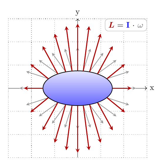
Graphical representation of the relationship between the angular velocity vector $\pmb{\omega}$ (gray) and the angular momentum vector $\pmb{L}$ (red) for an ellipsoid with inertia tensor $\mathbf{I}$. The directions of $\pmb{L}$ and $\pmb{\omega}$ do not coincide due to the anisotropy of the inertia tensor. The ellipsoid has dimensions 3, 1.5 and 1.5 along the x, y, and z axes respectively and is homogeneous in density.
5.7 Heavy symmetrical top with one point fixed:
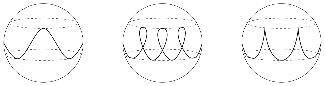
From left to right, monotone precession, spin-reversal precession and non-monotome precession.
6.2 water:
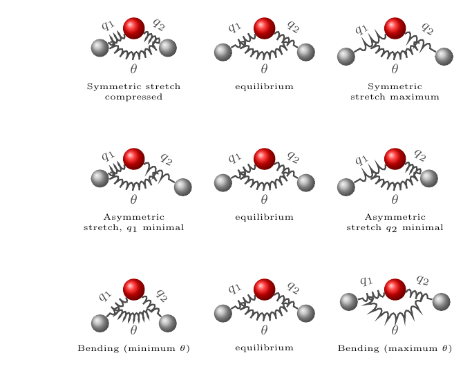
Vibrational modes of H$_2$O: 3N=9 degrees of freedom total. 3 vibrational (shown), 3 translational, 3 rotational. Modes: symmetric stretch ($q_1=q_2$), asymmetric stretch ($q_1 \neq q_2$), bending ($\theta$).
6.2 carbondioxide:
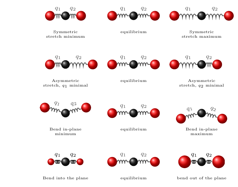
Vibrational modes of CO$_2$: 3N=9 degrees of freedom total. 4 vibrational (shown: symmetric and asymmetric stretch, bending in/out-plane), 3 translational, 2 rotational. Bending doubly degenerate (linear molecule). The springs between the C-O bonds and the corresponding generalized coordinate $\theta$ are omitted to avoid overloading the figure.
6.3 Normal Coordinates:
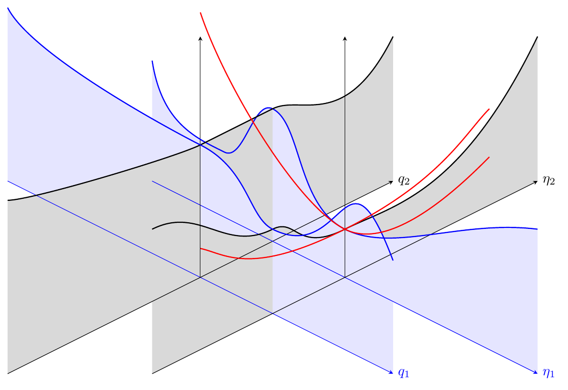
Expansion around a small diversion in a minumum up to second order.
8.1 Afbeelding1:
8.1 Slide 187b:
8.1 Slide 187: