Calculus III
1.2.3 Example evolute cycloid:
The cycloid $P(t)= \left[ R(t-\sin t), R(1-\cos t) \right]$ and its evolute $Q(t)= \left[ R(t+\sin t), R(\cos t - 1) \right]$, which is a translation of $P(t)$.
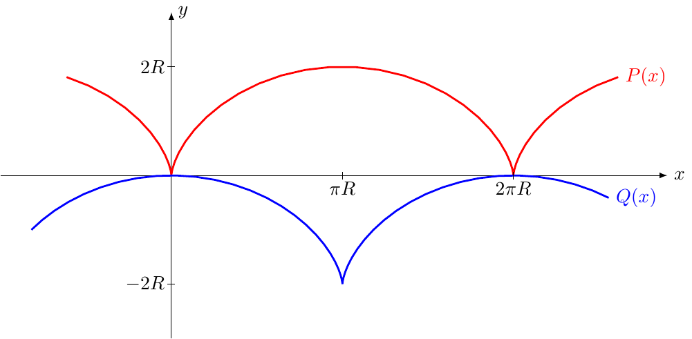
1.2.4 Example evolute catenary:
The catenary $P(x) = [x, a \cosh(x/a)]$ and its evolute $Q(x) = \left[x-\frac{a}{2}\sinh(2x/a), 2a \cosh(x/a)\right]$.
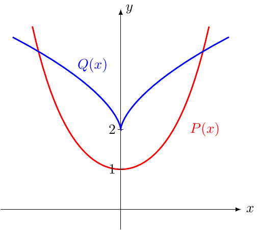
1.2.5 Example involute catenary (tractrix):
/standalone.PNG)
The catenary $P(x) = [x, a \cosh(x/a)]$ and its involute: the tractrix $Q(x) = \left[ x-a \tanh(x/a), \frac{a}{\cosh(x/a)}\right] $. For a point $Q$ on the tractrix, the intersection of the tangent to $Q$ with the $X$-axis coincides with the orthogonal projection of the corresponding point on the catenary $P$.
1.2.8 Example envelope family of straight lines:
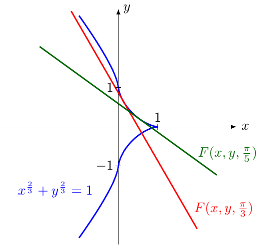
Some examples from the family of lines $F(x,y,a) = \frac{x}{\cos(a)} + \frac{y}{\sin(a)} = 1$, and the corresponding astroid: $x^{2/3} + y^{2/3} = 1$.
2.3 Gradient of scalar field:
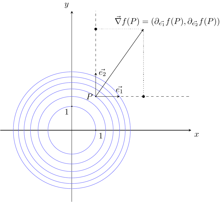
The scalar field $f(x,y)=x^2+y^2$ visualized by the planes $f(x,y)=n$ for $n\in {1,2,3,4,5,6}$. The gradient $\vec{\nabla} f(P)$ in a point P is given with its directional derivatives $\partial_i f(P) = \partial_{\vec{e}_i} f(P)$.
3.1 Line integral of a scalar field:
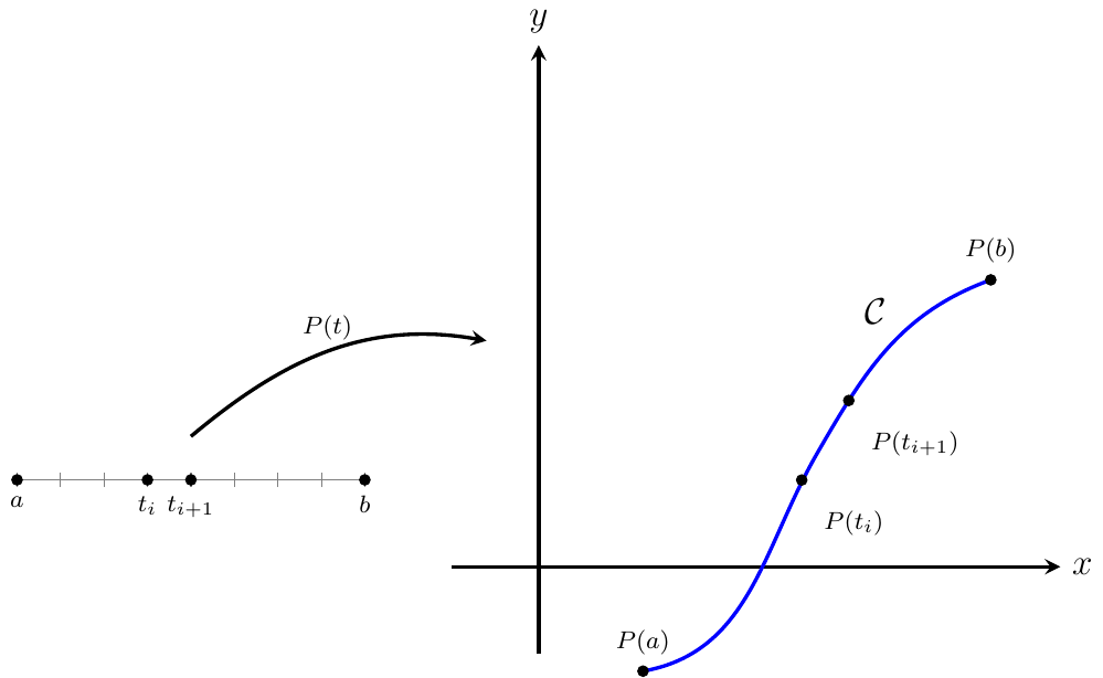
The line integral of a scalar field $\phi$ over a smooth curve $P(t)$ is given by: $\int_{\mathcal{C}} \phi ~ds := \int^b_a \phi \left(P(t)\right) \left\lVert \frac{\overrightarrow{dP}}{dt} \right\rVert dt.$ In the figure, the displacement between different points along the curve, $P(t_{i+1})-P(t_i)$, is shown. This relates to the infinitesimal displacement $\left\lVert \frac{\overrightarrow{dP}}{dt} \right\rVert dt$.
3.2 Line integral of a vector field:
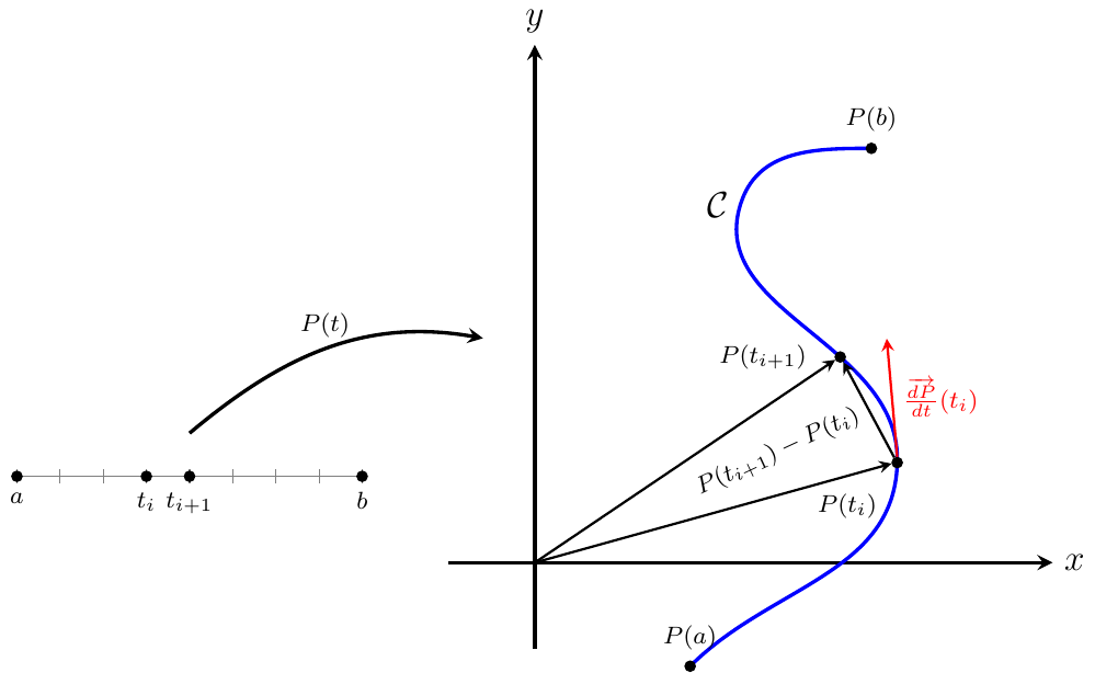
The line integral of a vector field $\overrightarrow{F}$ over a smooth curve $P(t)$ is given by: $\int_{\mathcal{C}} \overrightarrow{F} \cdot \overrightarrow{dP} := \int^b_a \overrightarrow{F} \left(P(t)\right) \cdot \frac{\overrightarrow{dP}}{dt} ~dt. $ In the figure, the displacement between different points along the curve, $P(t_{i+1})-P(t_i)$, is shown. This relates to the infinitesimal displacement vector $\frac{\overrightarrow{dP}}{dt} dt$.
3.4.2 Conservative field along a curve:
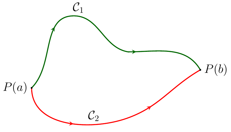
The points $A$ and $B$ lie on a closed curve $\mathcal{C}$. We can choose two arbitrary paths, $\mathcal{C}_1$ and $\mathcal{C}_2$, from $A$ to $B$. If we evaluate the line integral of a conservative field $\phi$ along both paths, the result will be the same, since the line integral of a conservative field is independent of the travelled path.
3.4.3 Proof conservative field:
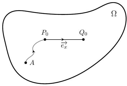
Proof that path-independence implies conservativeness in fields. Consider a path-independent vector field $\overrightarrow{F}$ in an open, connected region $\Omega$. A potential function $\phi(P_0)$ is constructed by integrating $\overrightarrow{F}$ along an arbitrary curve $\widehat{AP_0}$ from a fixed point $A$ to $P_0$. The path independence ensures that $\phi$ is well-defined, and its gradient reproduces $\overrightarrow{F}$.
3.5.1 Proof Greens theorem:
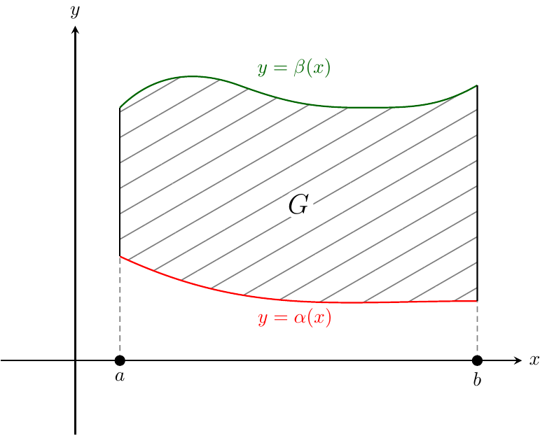
The normal region $G$ can be projected onto the x-axis, with its upper and lower boundaries parametrized by $y=\alpha(x)$ and $y=\beta(x)$.
3.5.2 Union of normal spaces:
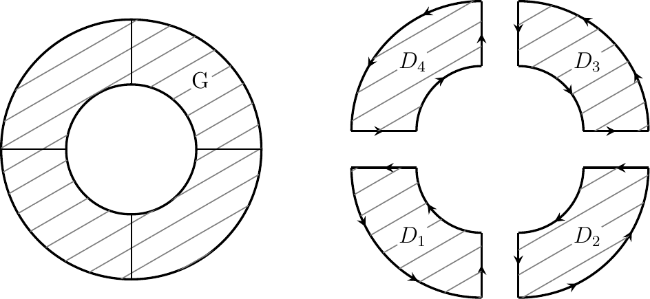
(Left) The annulus $G$ is not a normal region, as it cannot be projected onto the $X$- or $Y$-axis. (Right) However, $G$ is a union of normal regions: it can be split into four regions ($D_i$) each of which can be projected onto the $X$- and $Y$-axis.
3.5.4 Alternative formulation Greens theorem:
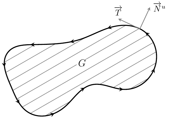
The alternative representation of Green’s theorem: $\int_{\partial G^+} \overrightarrow{F} \cdot \overrightarrow{N}^u ~ds = \int_G \overrightarrow{\nabla} \cdot \overrightarrow{F} ~dA,$ where $\overrightarrow{T}$ is the tangent unit vector and $\overrightarrow{N}^u$ the outward normal vector.
4.1 Surface integral of a scalar field:
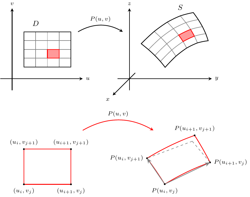
Construction of the surface integral of a scalar field $\phi$ over a smooth surface $S= P(u,v)$: $\int_S \phi ~d\sigma := \int_D \phi \left(P(u,v)\right) \lVert \overrightarrow{\partial_u P} \times \overrightarrow{\partial_v P}\rVert ~du ~dv$ (Below) An infinitesimal rectangle on $D$ with area $du_i ~dv_j$ is projected onto a curvilinear quadrilateral on $S$, which we can approximate by a parallelogram, with area: $\lvert \left(P(u_{i+1}, v_{j}) - P(u_{i}, v_{j}) \right) \left( P(u_{i}, v_{j+1}) - P(u_{i}, v_{j}) \right) \vert = \lVert\overrightarrow{\partial_u P(u_{i}, v_{j})} \times \overrightarrow{\partial_v P(u_{i}, v_{j})}\rVert ~du_i ~dv_j$. This is represented in the integral by the absolute value of the Jacobian determinant associated with the parameterization: $\lVert \overrightarrow{\partial_u P} \times \overrightarrow{\partial_v P}\rVert$.
4.4.1 The divergence theorem:
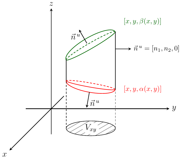
Proof of the divergence theorem. The normal region $V$ is projected onto the $XY$-plane, with projection $V_{xy}$. The upper and lower boundaries of $V$ are represented by a parametrization.
4.6.0 The corkscrew rule:
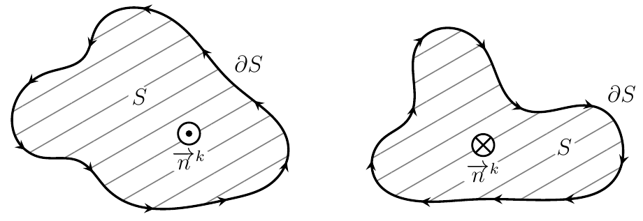
The unit vector along the surface normal, $\overrightarrow{n}^k$, is oriented such that its direction agrees with the orientation of $\partial S$ according to the corkscrew rule (or right-hand rule).
4.6.1 Stokes theorem:
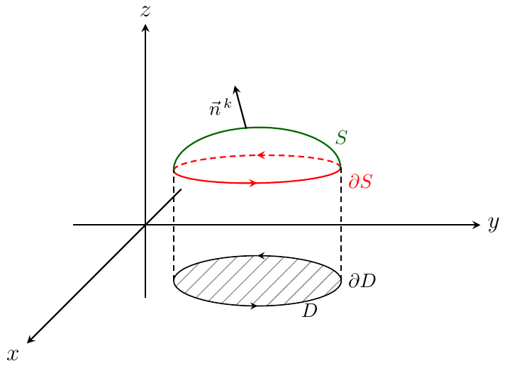
Proof Stokes’ theorem. $S$ is a smooth surface that can be projected onto the $XY$-plane, with projection $D$.
5.1 Inverse function:
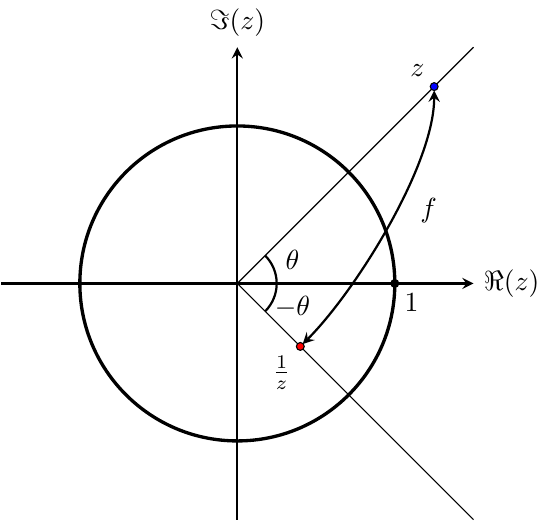
The reciprocal function $f(z)=\frac{1}{z}$ maps points outside of the unit circle inside the unit circle and vice versa. The ray with an angle $\theta$ will be mapped to a ray with angle $-\theta$.
5.1 Complex function:
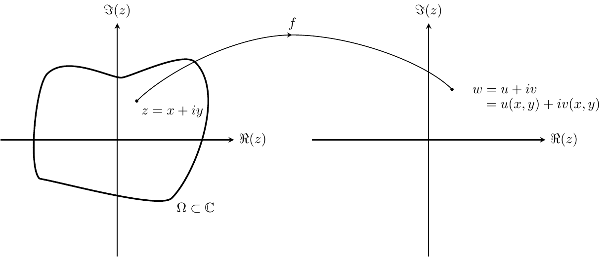
The complex function $f : \Omega \to \mathbb{C}$ which maps points from $\Omega \subseteq \mathbb{C}$.
5.2 Complex line integral:
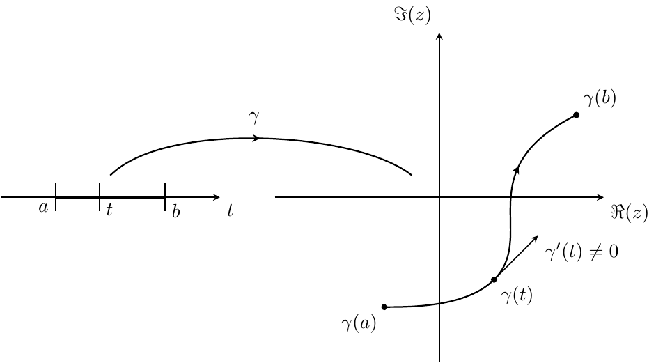
The complex line integral $\int_C f(z)\,dz$ for $z=\gamma(t)$, $t \in [a,b]$, with $\gamma(t)$ a smooth curve, can also be seen as an integral over $t$ with the equation $\int_C f(z)\,dz = \int_a^b f(\gamma(t))\,\gamma’(t)\,dt$
6.2.1 Complex derivative:
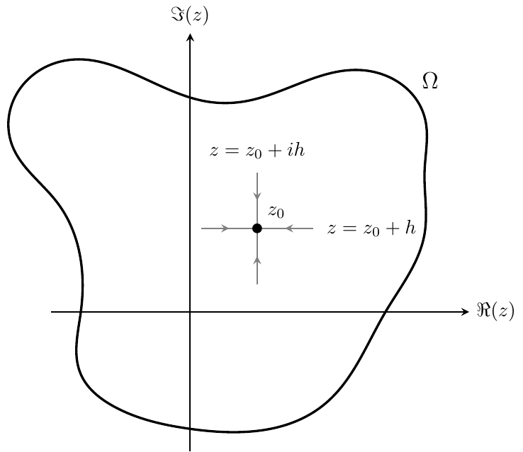
The complex derivative in a point $z_0 = x_0 + i y_0$ for a complex function is: $f’(z_0) = \lim\limits_{h \to 0} \frac{f(z_0 + h) - f(z_0)}{h}$. For $f’(z_0)$ to exist, this limit must be the same regardless of the direction in which $h \to 0$. In the figure, the limit is approached along the real and imaginary axes; equating the results of both approaches yields the Cauchy–Riemann conditions.
6.3 Cauchy Goursat theorem for multiply connected domains:
The integral over a contour $C$ in $\Omega$ with an interior with a finite amount of singular poles is the sum of the integrals over the circles around these interior poles.
6.3 Contour non simply connected:
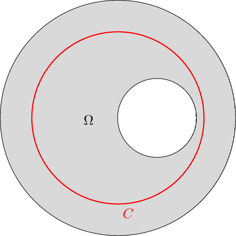
The interior region of $C$ does not lie entirely within $\Omega$. Wherefore we need information about the set of points not in $\Omega$.
6.3 Contour simply connected:
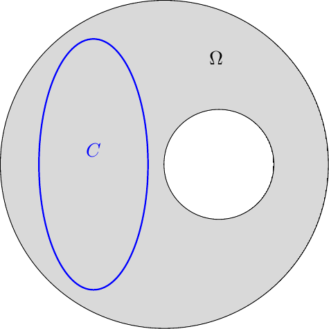
$C$ encloses a compact set that lies entirely within $\Omega$. In this case, the integral over the contour will be zero.
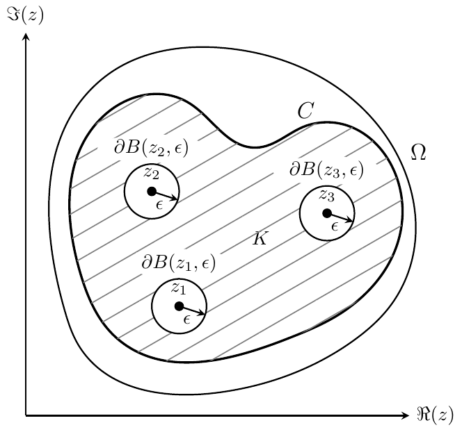
6.3.3 Proof integral formula Cauchy:
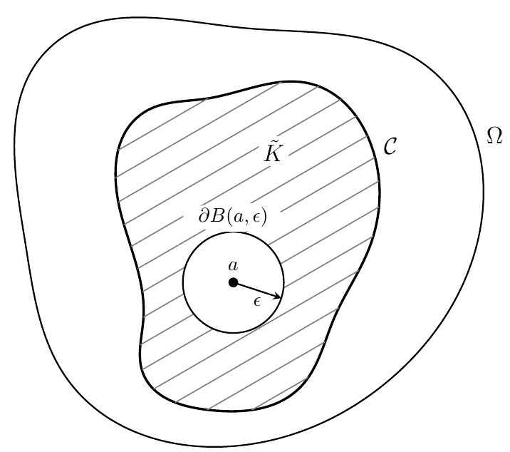
$\mathcal{C}$ is a bounded contour in $\Omega$ which encloses a compact set $K$ lying completely within $\Omega$. For a point $a \in \mathcal{C} \setminus K$, we parametrize the circle $\partial B(a, \epsilon)$, which lies entirely in the interior of $\mathcal{C}$.
7.2.4 Theorem convergence regions positive and negative power series:
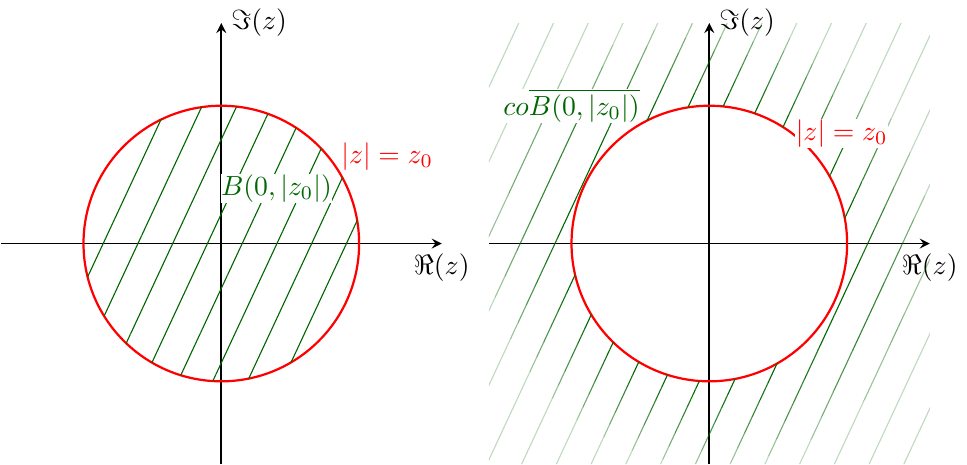
(Left) Region of convergence of a positive power series. (Right) Region of convergence of a negative power series.
8.2.1 Proof theorem Laurent series:
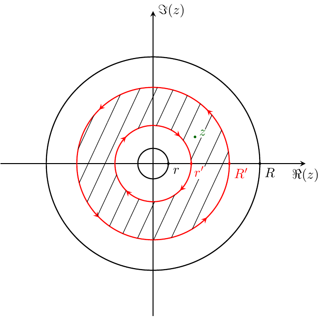
The region of convergence of the Laurent series is the annular region $ B(0, R) \setminus \overline{B(0, r)} $. For every point $ z $, it is possible to find $ R’ $ and $ r’ $ such that $ 0 < r < r’ < \lvert z \rvert < R’ < R. $
8.5.6 Residue theorem for region with multiple singularities:
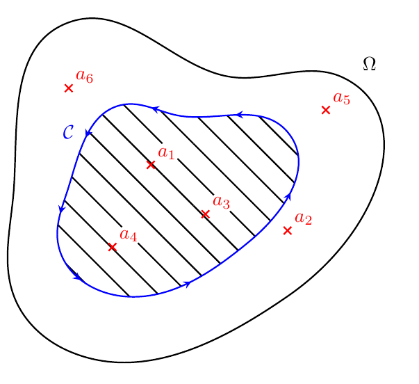
The contour $ \mathcal{C} $ passes through none of the singularities $ a_i $ of the complex function $ f $ and encloses a compact set that lies entirely within $ \Omega $. $ \mathcal{C} $ contains a finite number of singularities of $ f $.
9.3 Estimation lemmas:
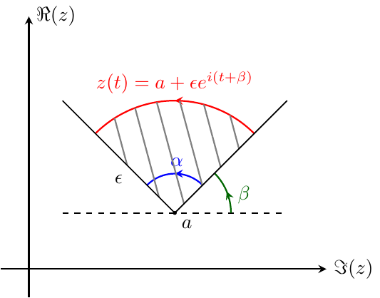
Small limit theorem: The circular arc $ C^{t}_{\varepsilon} $ with center $ a $, radius $ \varepsilon > 0 $, and central angle $ \alpha $ can be described by the parametric equation $z(t) = a + \varepsilon e^{i(t + \beta)}, \, t : 0 \to \alpha. $
9.5 Summation of series:
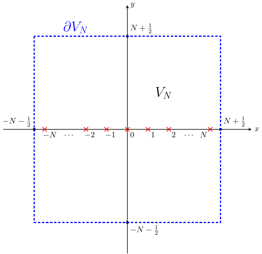
The function $ g(z) = \cot(\pi z) $ has simple poles at $ z = 0, \pm 1, \pm 2, \ldots $. If we consider the square $ V_N $ with center at the origin and side length $ 2N + 1 $, where $ N \in \mathbb{N} $, then we can compute the contour integral over $ \partial V_N^+ $ using the residue theorem.